Balancing Signal Integrity and Manufacturing Constraints in Industrial PCB Design

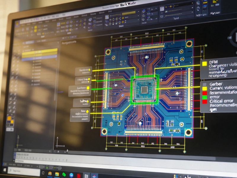
Industrial Pcb design lives in a constant tension. On one side, Signal Integrity demands wider traces for impedance matching, tightly controlled dielectric thicknesses, and layer stack-ups that prioritize return path continuity. On the other side, manufacturing reality imposes minimum trace widths, achievable etch tolerances, drill size limits, and cost boundaries that dont care about your eye diagram. Push too hard toward SI perfection and the board becomes unmanufacturable—or manufacturable only at a price nobody will pay. Ignore SI constraints and the board may pass electrical validation in the lab but fail intermittently in the field when noise margins erode under real-world conditions. Finding the balance is what separates a design that works on paper from one that works in production, reliably, at scale. This article explores the key tradeoffs and practical strategies for balancing Signal Integrity with manufacturing constraints in Industrial Pcb design.

The Core Conflict: What SI Wants vs. What Fabrication Can Deliver

Signal integrity requirements and manufacturing capabilities pull in opposite directions on several fundamental parameters:

• Trace width and spacing: SI wants 50-ohm Microstrip traces that might be 5–7 mils wide on thin dielectric—but your fabricators minimum finished trace width might be 4 mils with a ±1 mil etch tolerance. That tolerance band creates impedance variation that directly degrades signal quality.
• Dielectric thickness control: Controlled Impedance requires tight dielectric thickness between signal and reference layers. A ±10% variation in prepreg thickness (which is normal for standard FR-4 processes) can shift impedance by 5+ ohms on a 50-ohm target.
• Via transitions: Every layer transition introduces stub length, parasitic inductance, and return path disruption. SI wants back-drilling or HDI blind/buried vias to eliminate stubs; manufacturing adds cost and cycle time for each back-drill operation.
• Layer count: More layers give you dedicated reference planes and signal routing room—but every additional layer pair increases cost, lead time, and lamination risk.

Understanding these conflicts is the first step. The next step is knowing which compromises are acceptable and which will bite you in production.

Stack-Up Design: Where SI and DFM Collide First

The layer stack-up is where the balance between signal integrity and manufacturing constraints is most visible—and most consequential. A well-designed stack-up simultaneously satisfies impedance targets, provides adequate return paths, and stays within what your fabricator can actually build with acceptable yield.

Impedance-Controlled Stack-Ups for Industrial Speeds

Industrial PCBs increasingly operate at speeds that demand Controlled Impedance. Motor drive control loops run switched frequencies of 100kHz+ with fast edges that contain harmonic content well into the hundreds of MHz. Industrial Ethernet, PROFINET, and EtherCAT interfaces run at 100Mbps or 1Gbps. Industrial vision systems and high-speed data acquisition push into multi-gigabit territory.

For these applications, a stack-up must deliver:

• Consistent reference planes: Every signal layer needs an adjacent continuous ground or power plane for return current. A signal0 signal layer sandwiched between two other signal layers is an SI disaster, regardless of trace geometry.
• Target impedance with achievable geometry: Calculate trace widths based on your fabricators actual dielectric constants and thicknesses—not textbook nominal values. Request impedance coupons on production panels and specify ±10% tolerance at minimum.
• Symmetric construction: A balanced stack-up (same dielectric thickness and copper weight above and below the center core) prevents board warpage during lamination and reflow. Warped boards cause assembly defects and connector mating problems in industrial enclosures.

A practical 6-layer industrial stack-up for mixed-signal designs might look like: Top Signal (Microstrip) / Ground / Power / Signal (Stripline) / Ground / Bottom Signal (microstrip). This gives three signal layers each adjacent to a reference plane, with symmetric outer dielectric thicknesses. The Stripline layer on L4 is ideal for critical clock and high-speed Differential Pairs that need the best isolation from both EMI ingress and egress.

The Prepreg Thickness Trap

Here is a manufacturing detail that catches many designers off guard: prepreg thickness is not1 not a single, controlled value. Prepreg is glass fiber cloth impregnated with partially cured resin, and its thickness after lamination depends on the copper fill on adjacent layers, the press cycle pressure, and the resin content of the specific prepreg style.

A "106" style prepreg might be listed as 3.5 mils nominal in a datasheet, but after lamination over heavy copper planes with minimal etching, it compresses to perhaps 2.8 mils. Over sparse copper with lots of etched gaps, it flows into the voids and the effective dielectric between trace and reference plane ends up thicker—maybe 4.2 mils. That variability directly impacts impedance.

The mitigation: work with your fabricator to get their measured post-lamination dielectric thickness data for the specific stack-up you are using. Specify copper fill patterns (thieving or shadow plating) to make copper distribution uniform across layers, which reduces prepreg thickness variation. Its a manufacturing step that directly improves SI consistency.

Trace Geometry: Finding the Manufacturable Sweet Spot

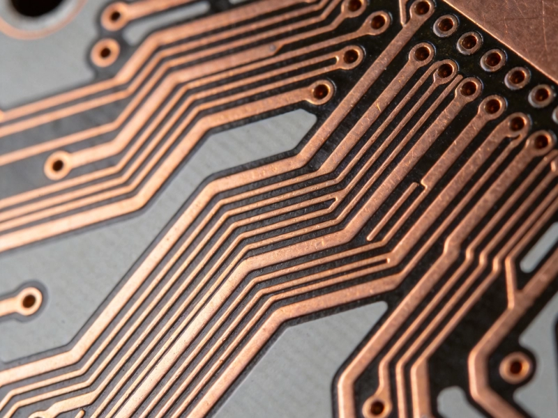
Controlled impedance trace geometry is where the SI-vs-manufacturing tension gets very concrete. You calculate that a 50-ohm microstrip trace on your stack-up needs to be 4.2 mils wide. Your fabricator says they can do 4 mil minimum but with ±1 mil etch tolerance. That means your actual trace width in production could be anywhere from 3.2 to 5.2 mils—and your impedance could swing from roughly 44 to 56 ohms.

Strategies to Widen Traces While Maintaining Impedance

If minimum trace width is causing Impedance Control problems, you have several options:

• Use a thicker dielectric: Moving from a 3.5-mil prepreg to a 5-mil prepreg between the signal layer and its reference plane increases the trace width needed for 50 ohms. Wider traces have better etch tolerance as a percentage of width, improving impedance consistency.
• Use embedded microstrip (coplanar with ground): Adding ground copper adjacent to the trace at a controlled spacing creates a coplanar waveguide structure that can achieve 50 ohms with wider traces on thinner dielectric. The catch, the spacing to ground must also be controlled, so you need tighter etch tolerance on the spacing dimension too.
• Switch to stripline: Stripline traces (embedded between two reference planes) typically require wider traces for the same impedance compared to microstrip, which gives you more manufacturing margin. They also have better isolation and no far-field radiation, which is valuable for noisy industrial environments.

Differential Pair Routing Tradeoffs

Differential Pairs for industrial high-speed interfaces (USB, PCIe, Gigabit Ethernet) add another dimension to the trace geometry challenge. The differential impedance depends on both the trace width and the pair spacing. Tight coupling (small spacing) provides better noise rejection and EMI performance but makes the pair more sensitive to etch variation on the spacing dimension.

A pragmatic approach for industrial PCBs:

• Use loosely coupled differential pairs where possible—spacing of 2× to 3× the trace width. This makes differential impedance less sensitive to manufacturing variation at the cost of slightly reduced common-mode rejection. For most industrial speeds (below 5Gbps), the noise margin budget can absorb this tradeoff.
• Specify pair matching as time delay, not length matching: Manufacturing variation in trace width affects propagation velocity. Two traces of identical length but different width (due to etch variation) have different propagation delays. Specifying ±5ps skew instead of ±10mil length match accounts for this reality.
• Route pairs on the same layer: Never split a differential pair across layers if you can avoid it. Via transitions introduce impedance discontinuities and can be different between the positive and negative legs, creating mode conversion.

Via Strategy: The Layer Transition Problem

Vias are necessary for routing connectivity but they are the enemies of signal integrity. Every via is an impedance discontinuity, a return path interruption, and a potential radiation source. In industrial PCBs with mixed-signal architectures—where a power stage switching at 100kHz+ shares the board with sensitive analog measurement circuits—via strategy can make or break system performance.

Through-Hole Via Limitations

Standard through-hole vias in a 1.6mm or 2.4mm Industrial Pcb create stubs when used for layer transitions that dont span the full board thickness. A via transitioning from L1 to L2 in a 6-layer board leaves a 4-layer stub that resonates at frequencies where the stub length is a quarter wavelength. For a 1.2mm stub in FR-4, that resonance falls around 35GHz—well above most industrial signal speeds. But the stub still contributes capacitive parasitics that degrade edge rates and create reflection coefficients of 5–10% at gigabit speeds.

Back-Drilling: Manufacturable Stub Removal

Back-drilling (also called controlled depth drilling) removes via stubs by drilling from the opposite side of the board to a controlled depth after plating. Its the most manufacturable approach to stub elimination for layer counts up to about 12 layers.

Key manufacturing constraints for back-drilling:

• Depth tolerance: Typical back-drill depth tolerance is ±3 mils. The drill must penetrate past the target layer without damaging the next layer. This requires minimum 5-mil spacing between the target stop layer and the next layer.
• Cost impact: Each back-drill setup adds a drilling pass. For a board with two different stub lengths (e.g., vias from top to mid, and vias from bottom to mid), thats two additional drill passes. Cost increase is typically 10–20% over standard drilling.
• Registration accuracy: Back-drill registration must align with the original via locations. Misalignment can clip via barrels partially, creating reliability risks. Your fabricator needs to confirm their registration capability matches your via pitch and density.

HDI Vias: When Through-Hole Isnt Enough

For high-density industrial boards with BGA-packaged FPGAs or processors, HDI via structures (blind and buried vias) provide the layer transition capability without stubs. A Blind Via from L1 to L2 is typically 4–6 mils in diameter and only penetrates the outer dielectric layers—no stub at all.

However, HDI adds significant manufacturing complexity:

• Sequential Lamination: Blind and buried vias require multiple lamination cycles, increasing both cost and cycle time. A 1-n-1 HDI structure (one Blind Via layer on each side) doubles the lamination steps.
• Via fill and planarization: Blind Vias under BGA pads must be filled with copper or epoxy and planarized flat for solderability. This adds plating and grinding processes that have their own yield impacts.
• Reliability concerns: The Microvias in HDI structures are more susceptible to fatigue failure under Thermal Cycling than through-hole vias, particularly at the capture pad interface. Ipc-6012 class 3 (high reliability) industrial applications require careful qualification of HDI via reliability.

The decision framework: use through-hole vias with back-drilling for industrial boards running at speeds up to about 5Gbps. Reserve HDI for boards that need both high routing density and speeds above 5Gbps where via stubs and transition discontinuities cannot be tolerated.

Return Path Continuity: The Manufacturing Challenge Nobody Talks About

Signal integrity fundamentals say that return current flows on the reference plane directly beneath (or above) the signal trace. This works perfectly when the reference plane is continuous. In real industrial PCBs, reference planes get fragmented by mounting holes, connector cutouts, via antipads, and plane splits for power domains. Each discontinuity forces return current to detour around the obstacle, creating a loop area that radiates EMI and increases crosstalk to adjacent signals.

Practical Return Path Management

Maintaining return path continuity while meeting mechanical and Power Distribution requirements takes deliberate effort:

• Via antipad management: Each signal via creates an anti-pad (clearance) in every plane it passes through. In dense via fields—like under a BGA fan-out—these anti-pads can merge and cut entire channels through a ground plane. Minimize anti-pad diameter and avoid overlapping anti-pads by staggering via placement. A 20-mil anti-pad versus a 30-mil anti-pad makes a significant difference in how much copper remains between vias.
• Bridge the gaps: When a signal trace must route over a plane slot (for example, crossing between two power domains), place stitching vias on both sides of the slot where the trace crosses. These vias provide return current a path to flow from one side of the slot to the other, minimizing the loop area discontinuity.
• Mounting hole placement: Industrial PCBs need mounting holes for mechanical stability. Keep mounting hole keep-out zones away from high-speed signal routing layers. When a mounting hole must be near high-speed traces, ensure the ground plane void around it is as small as the mechanical hardware allows.

These return path considerations dont show up in schematic-level SI analysis—they only emerge in layout. That is why SI review of the physical layout is essential for industrial boards, not just the topology and length matching.

Material Selection: Where Performance Meets Processability

The PCB laminate material affects both signal integrity and manufacturing yield. Higher-performance dielectrics have lower loss tangent (better for high-speed signals) but often come with manufacturing challenges.

Standard FR-4 vs. Low-Loss Materials

For industrial PCBs operating at frequencies below about 2GHz, standard FR-4 (Df ≈ 0.02) is usually adequate from a loss perspective. The attenuation over typical board trace lengths of 6–12 inches is manageable. Above 2GHz—common for industrial Ethernet backplanes, high-speed serial links, and millimeter-wave radar sensors—standard FR-4 Insertion Loss becomes prohibitive.

Low-loss laminates (Df ≈ 0.005–0.010) solve the loss problem but introduce manufacturing considerations:

• Drill wear: Low-loss materials often use ceramic or PTFE-based resin systems that are abrasive and wear drill bits faster. Your fabricator needs to adjust drill feeds and speeds, and expect more bit changes per panel. This affects both cost and hole wall quality.
• Lamination cycles: Some low-loss materials require different lamination temperature and pressure profiles than standard FR-4. Mixed-dielectric stack-ups (standard FR-4 core with low-loss prepreg) need lamination parameters that work@ that satisfy both materials, which can be tricky to dial in.
• Copper adhesion: PTFE-based laminates have notoriously poor copper adhesion. Special surface treatments (sodium etch or plasma treatment) are. are required before copper plating. If your fabricator doesnt have this capability, you will get peeling copper during Thermal Cycling.
• CTE mismatch: Some low-loss materials have CTE values significantly different from standard FR-4. In mixed-material stack-ups or when using lead-free assembly (peak reflow 260°C), the thermal expansion mismatch can cause Delamination or via barrel cracking.

The practical recommendation for industrial designs: use a mid-tg, low-Df laminate (like a modified epoxy system with Df around 0.010) as your baseline. It provides meaningful loss improvement over standard FR-4 without the severe manufacturing challenges of full PTFE systems. Reserve full PTFE or ceramic laminates for applications where nothing else meets the electrical requirements.

Design for Manufacturability Checks That Preserve Signal Integrity

Dfm Review often gets treated as a separate step from SI review, with DFM pushing for wider traces, bigger vias, and more spacing while SI pushes for tighter geometries. The best results come from running DFM and SI checks together and resolving conflicts jointly rather than sequentially.

Integrated DFM-SI Checklist for Industrial PCBs

• Trace width vs. impedance target: Verify that calculated trace widths for target impedance are above the fabricators minimum +2× etch tolerance. If not, adjust dielectric thickness or consider stripline routing.
• Spacing vs. crosstalk budget: Check that trace-to-trace spacing meets both the fabricators minimum spacing and the crosstalk isolation requirement for the signals involved. Dense routing between slow signals can use minimum spacing; high-speed pairs need wider separation.
• Via diameter vs. pad size: Ensure via pad diameter is at least 18 mils larger than the drill diameter for reliable annular ring. For impedance-controlled nets, verify that the via pad size doesnt create an impedance bump larger than your reflection budget allows.
• Plane clearance vs. return path: Verify that anti-pad sizes and plane cutouts dont fragment reference planes beyond what return path continuity requires. Run a plane integrity check in your layout tool.
• Impedance test coupons: Include impedance test coupons on the production panel for every unique impedance value in the design. This is both a manufacturing requirement (for process verification) and an SI requirement (for correlation between as-built and as-designed impedance).

Manufacturing Tolerance Budgeting for SI

Signal integrity analysis typically uses nominal values for trace width, dielectric thickness, and Dk. In production, every parameter has a tolerance band. The disciplined approach is to run SI analysis at both nominal and worst-case corners:

• Best case: Minimum trace width, minimum dielectric thickness, minimum Dk (highest impedance, fastest edge rate)
• Worst case: Maximum trace width, maximum dielectric thickness, maximum Dk (lowest impedance, slowest edge rate)

If both corners pass your eye diagram, timing margin, and crosstalk budget, then manufacturing variation wont cause field failures. If one corner fails, you know exactly which parameter to tighten—and can make an informed decision about whether tighter fabrication tolerance (higher cost) or relaxed SI margin (performance risk) is the right tradeoff for your application.

Real-World Industrial Design: A Practical Example

Consider a typical industrial motor controller PCB: a 6-layer, 2.0mm board with a 1200V IGBT power stage, gate driver circuits, current sensing amplifiers, and a 100Mbps EtherCAT communication interface. This design embodies the SI-manufacturing balance challenge:

• Power stage layout: The IGBT and gate driver require wide copper traces for current capacity and thermal conduction. These wide traces (100+ mils) create large capacitive loads and radiate switching harmonics. The SI solution—keeping gate drive loops small with tight trace-to-return-path spacing—is compatible with manufacturing but requires careful plane management near the high-voltage clearance boundaries.
• Current sensing: The analog current sense amplifiers need quiet ground references and short connections to sense resistors. Trace widths of 8–10 mils are adequate for current but must maintain distance from the switching nodes. Manufacturing has no issue with these geometries—the challenge is purely placement and routing discipline.
• EtherCAT interface: 100Mbps differential pairs with 100-ohm differential impedance. On a 2.0mm board with standard FR-4, achieving 100-ohm differential impedance with manufacturable trace widths (6+ mils) is straightforward. The key SI requirement—length matching within 500mils—is easily achievable. The manufacturing concern is ensuring that the Ethernet transformer and connector footprints meet both the mechanical assembly requirements and the return path continuity needs.

This example illustrates that most industrial SI challenges are not about exotic materials or impossible geometries—they are about consistent application of fundamentals within the constraints of what your fabricator and assembler can reliably deliver.

Key Takeaways

• The tension between SI requirements and manufacturing constraints is fundamental in industrial Pcb Design—neither can be optimized in isolation.
• Start with a stack-up that satisfies both impedance targets and symmetric construction for manufacturing reliability.
• Choose trace geometries that achieve target impedance with margin for etch tolerance—dont design at the fabricators absolute minimum.
• Via strategy must account for stub effects, return path continuity, and the cost-reliability tradeoff between through-hole, back-drilled, and HDI via structures.
• Material Selection should balance electrical performance with processability—mid-range low-loss laminates often provide the best tradeoff for industrial applications.
• Run DFM and SI reviews jointly, not sequentially, to resolve conflicts at the root rather than with band-aids.
• Budget manufacturing tolerance into your SI analysis—if your design only works at nominal values, it wont work reliably in production.

Designing an Industrial Pcb that meets signal integrity targets and is reliably manufacturable isnt about finding a single perfect compromise—its about making informed tradeoffs at every decision point, with full knowledge of what each choice costs on both sides of the balance. When your boards pass electrical validation, pass production impedance testing, and survive thermal cycling in the field, you have found the right balance.

Contact us to discuss your requirements